Much of so called scientific evidence that is cited in the media is based upon a correlation of two variables. Thankfully, many of us are aware that correlation does not imply causation. However, this doesn’t completely stop us from using correlational evidence to establish or believe in a causal relationship. And this is for two key reasons.
First, it is easy to measure correlation between two variables and therefore tempting to arrive at premature conclusions of causality. We’re basically lazy.
Second, we usually possess good rationale or intuition, especially when it comes to figuring the direction of the causal effect. For example, if we observe that there is a positive correlation between years of schooling and wages, we are usually prepared to state that education causes wages to go up because there is a very compelling theoretical rationale that a person’s wage is a function of skills and experience. So the direction of the causal effect may indeed be positive as we intuited. However, any contributions from correlational evidence would stop there because we’re also very much interested in quantifying the magnitude of the causal effect – not just the direction. We want to be able to answer such a question: by how much do years of schooling impact a person’s wage? Unfortunately, correlational evidence does very little if anything to accurately estimate the magnitude of the causal relationship, which is why it’s imperative that we use causal inference to correctly deduce not only the direction of the causal relationship, but also the magnitude.
Covariance and correlation are two statistical measurements of correlation (linear association) between two variables. Despite the similarities between these two terms, formulaically they are different from each other and used in different contexts. The following points are noteworthy so far as the difference between covariance and correlation is concerned:
Covariance is a measure used to indicate the extent to which two variables change in tandem. Covariance is affected by the change in scale, meaning that covariances are hard to compare. When you calculate the covariance of a set of heights and weights expressed in meters and kilograms, we will get a different covariance from when we do it in imperial units (feet and pounds). Therefore, if we ever compare covariances calculated using the two different units of measurement, it would be hard to tell if the height and weight of people in Britain covary differently than those of people in Japan simply because covariance is not scale invariant.
The solution to this is to normalize covariance by dividing covariance by a term that represents the variance (measure of spread) in both the X and Y variables, and end up with a value, correlation, that is assured to be between -1 and 1. Whatever unit our original variables were in, we will always get the same result, and this will ensure that we can, to a certain degree, compare whether two variables correlate more than two others, simply by comparing their correlation.
To summarize, correlation is scale invariant. The value of correlation will always take place between -1 and +1. Conversely, the value of covariance lies between -∞ and +∞ and is influenced by scale. When it comes to considering which is a better measure of the relationship between two variables, there is no obvious answer. Correlation is preferred over covariance when we don’t care about the scale or magnitude of the relationship. But when the magnitude matters, then covariation can come in usefully.
Note that covariance is the numerator and the denominator is the normalizing constant that assures that the resulting division is between -1 and 1.
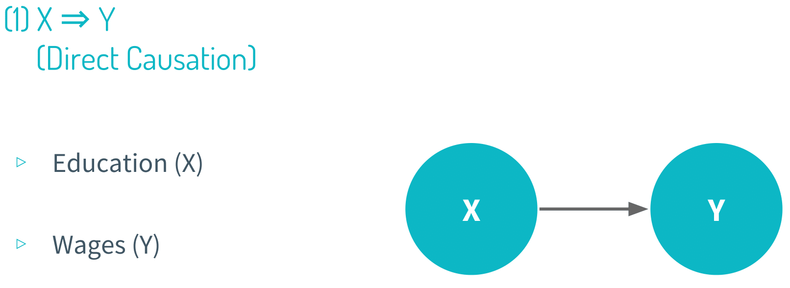
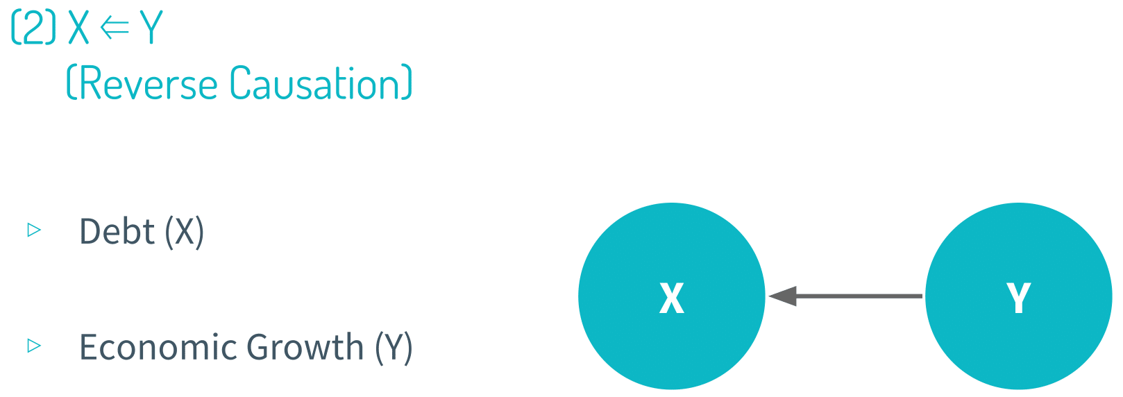
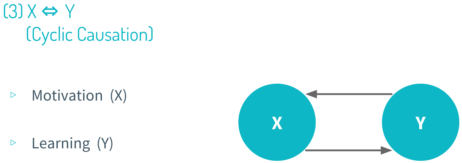
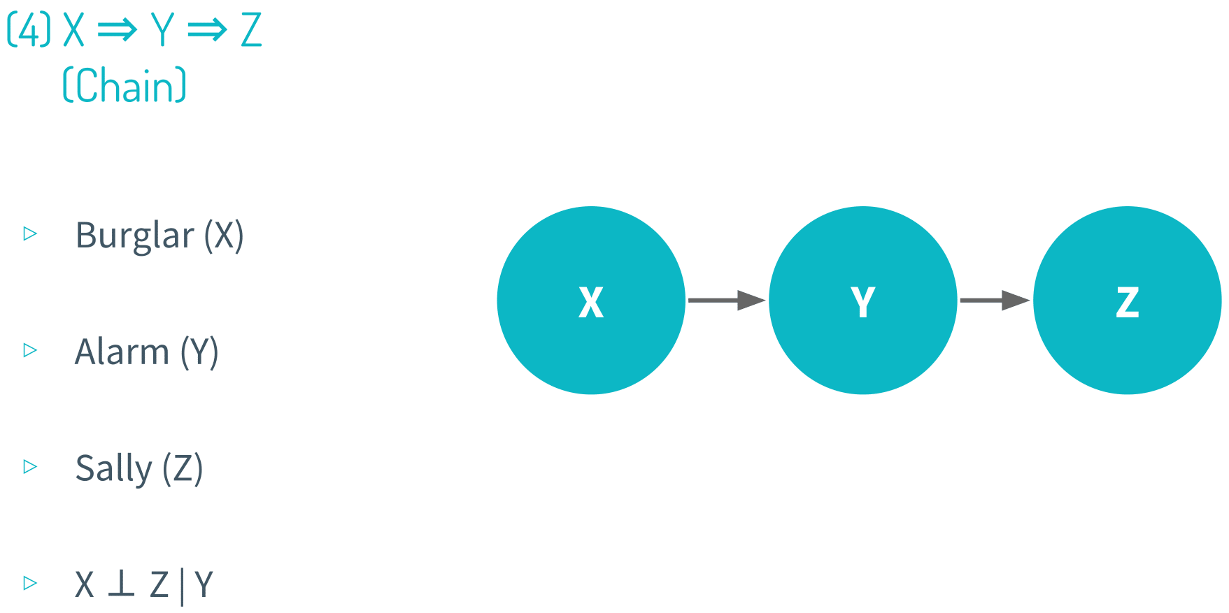
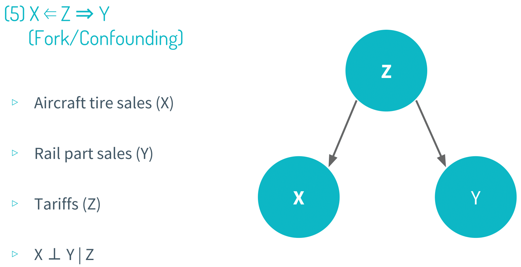
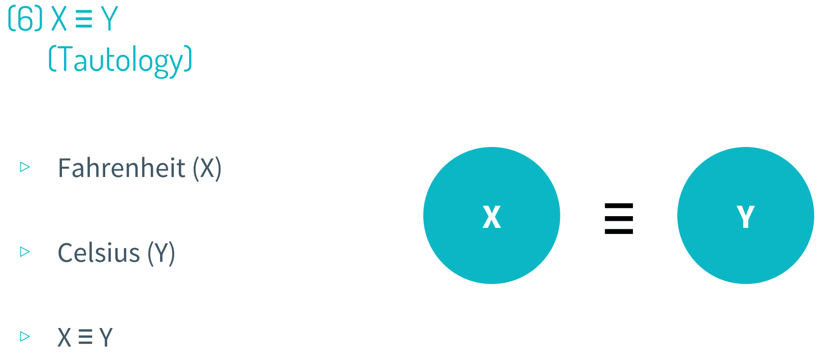
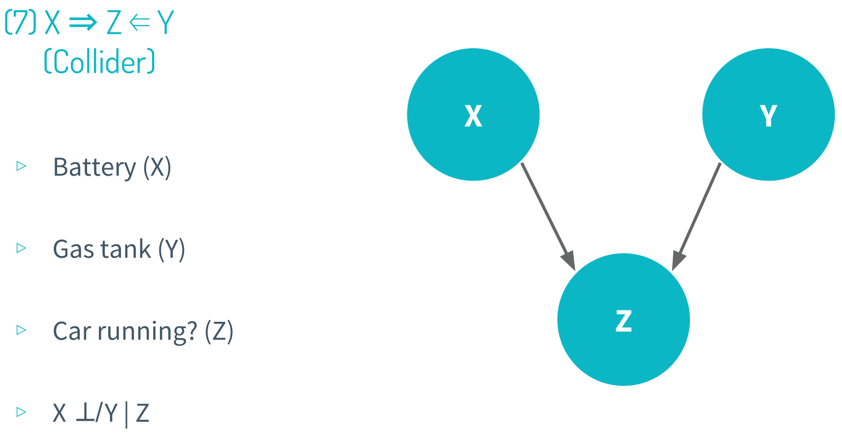
Graphical representations are often used to theorize the relationship between a set of variables. And in this module,we showed 8 canonical correlational structures to show the characteristics of each type.
Note that all of these visual representations are theoretical, meaning that when we are studying the relationship between a set of variables (X, Y, Z and so on), we don’t know what their relationship with one another looks like. And this is precisely why we use causal inference in the first place; our goal is to procure evidence to say whether the relationship is reverse causation, chain, collider or any other type.

It’s always important to keep in mind the five causality checks. Time order is pretty obvious. Variation in X has to occur before variation in Y for X to be a causal variable and Y to be an effect variable. This is purely definitional, so it becomes almost trivial to point this out.
Then there is covariation, which means that there must be a measurable statistical association between two variables. This requirement is also definitional because by hypothesizing that there is a causal relationship between X and Y, we are necessarily supposing that X and Y have a statistical association (they covary). Otherwise X and Y would appear to be independent variables, which is evidence that X and Y may not have a causal relationship.
Next there is significance, which means that our estimation of the true causal effect of X on Y must not be due to sampling error alone. In statistics, sampling error is when the characteristics (parameters) of a population are estimated from a subset or sample of that population. Since the sample does not include all members of the population, characteristics of the sample, such as means, medians and quantiles will generally differ from the characteristics of the entire population. For example, if we measure the heights of one hundred individuals from a country of twenty million, the average height of the thousand will most likely not be the same as the average height of all twenty million people in the population. Since sampling is typically done to infer the characteristics of a whole population, the difference between the sample and population characteristics is considered an error, a sampling error.
Similarly, in any social science study that involves drawing and studying a sample from a population, there is always the possibility that an estimated causal effect would have occurred due to sampling error alone. The mathematics involved in the statistical tests to show that the estimate of the causal effect is real and not due to sampling error are outside the scope of the course. But it’s important to be wary that social scientists, at least the serious ones, always use statistical methods to quantify and make note of the significance of the results in order to say whether the estimate of the true (population) causal effect are significant.
We also have to develop a rationale for a causal relationship between a set of variables. This is an underrated requirement in the causality checklist because it comes as obvious to most of us that there must be a logical compelling explanation behind a causal relationship.
The last thing on the checklist is to check for non-spuriousness, which means that we have to be sure that it’s the variation in X that causes the variation in Y, and nothing else. There can’t be a variation in W, or some other variable that is actually causing the variation in Y. Simply put, rival explanations must be ruled out. It turns out that eliminating rival explanations is one of the hardest checks we have to accomplish in our causal inference checklist, which is why researchers will usually devote most of their time explaining how their methodology controls for other factors. Controlling for other factors is commonly known as ceteris paribus.
Ceteris paribus is a Latin term that means all other things held constant or nothing else changes. For example, we might say, “As the price of Kit Kat rises, the quantify demanded of Kit Kat falls, ceteris paribus.” What does this mean?
If we raise the price of Kit Kat, and nothing else changes - people’s preference do not change, the recipe for Kit Kat do not change, and so on - then in response to the higher price of Kit Kat, people will buy less Kit Kat.
Suppose we have started eating fat-free ice cream for the past two months but failed to lose any weight. Does that mean eating fat-free ice cream (instead of regular ice cream) won’t help us lose weight?
Not at all. We know that eating fat-free ice cream will help us lose weight assuming nothing else changes or ceteris paribus. In other words, if we were eating one bowl of regular ice cream twice a week, and we now replace it with one bowl of fat-free ice cream twice a week, and we change nothing else (hold constant or fixed) - we don’t change how much we exercise, or how much we eat, and so on - then replacing regular ice cream with fat-free ice cream (in due time) will cause us to lose weight.
In social sciences, we are interested in estimating the average treatment effect because of two main reasons. First, it’s impossible to calculate the unit level treatment effect because we cannot compare a person’s outcome in both states, with treatment and without treatment (i.e. control). To do so ceteris paribus would require simultaneously receiving treatment and control and measuring both the treatment outcome and the control outcome, which is impossible to do. Borrowing the Frostian metaphor, a person cannot both take the road less traveled by and the road more traveled by. A person will invariably commit to a decision (treatment or control), which leaves us with only one observed outcome and a theoretical counterfactual outcome.
Secondly, most treatments are designed to treat more than just one person, which means that average causal effects are much more relevant - at least in the context of social sciences - than unit level treatment effects. Besides, we also know that calculating unit level treatment effects are unfeasible. How convenient!