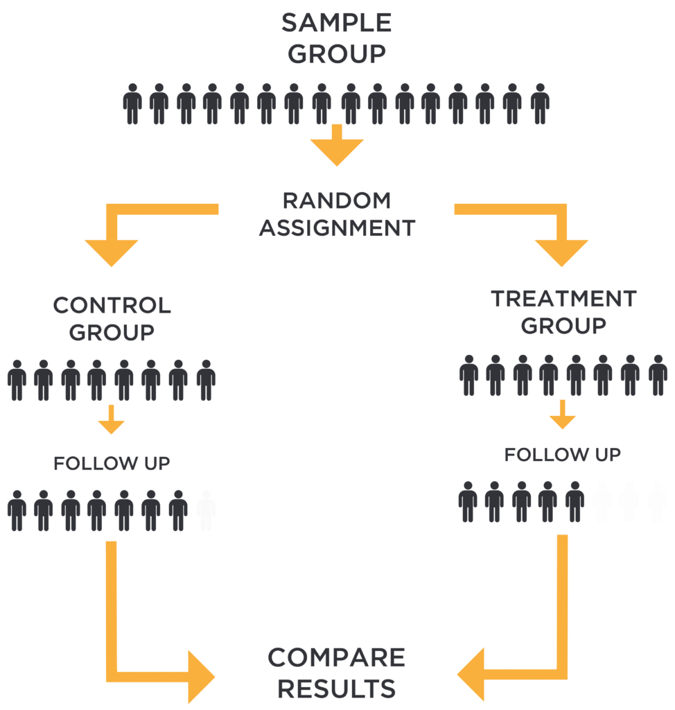
Randomized experiments are called the “gold standard” of causal inference because if done properly, the causal effect we derive from the experiment is robust to a lot of the faults that other techniques suffer from. So what is a randomized experiment? There are four components:
(1) There is a treatment to be studied like a policy, program, a drug, or more broadly and simply, a treatment.
(2) There is a treatment group that receives a treatment. There is also a control group. Sometimes, this is a group that doesn’t get any treatment at all, and other times it is a group that gets some other kind of treatment, but of a different kind or smaller amount.
(3) Now here’s the focal point. The subjects in our study must be randomly assigned to either a treatment or control group. It is critical that nobody – neither the researchers nor the people in the experiment – can participate in the decision about which group people fall into. Some kind of randomization procedure is used to put people into groups – flipping a coin, using a computer or some other method. This is the only way we can make sure that the people who get the intervention will be similar to those who do not. Referring to the ceteris paribus condition - holding all factors constant or equal - we want these two groups of people to be similar in all aspects (observed and unobserved), such that the difference in outcomes is solely attributed to the difference in treatment status between the two groups of people. Put it another way, the control outcome becomes the counterfactual outcome of the treatment group - what would have happened to the treatment group had they not received the treatment. This is how we can derive the causal effect of the treatment.
(4) There must be carefully defined outcome measures, and they must be measured before and after the treatment occurs. We measure before and after the treatment so that we have measured change in actual units, instead of relying on impressions or memories.
The idea behind controlled regression is that we want to control directly for confounding variables in a regression of Y on X by including them in our regression model as control variables. This idea of controlling for variables goes back to the ceteris paribus condition. We only want to know the causal effect of the treatment on the outcome variable, which means that the variation in other things should be controlled for (held constant).
We’d like to capture every relevant variable that can bias the causal effect of the treatment variable on the outome variable, but in practice, we know we cannot observe every single relevant variable. We can’t control for everything,which is what ceteris paribus means: all else equal. So do we give up on ceteris paribus? Well not necessarily. The key question that every user of controlled regression has to answer is this: have enough key factors been controlled for, or made equal across comparison groups, such that bias from the things we haven’t accounted for is mostly eliminated. This is also called the Unconfoundedness Assumption. And admittedly, this is really hard to argue and rationalize, because we have to convince ourselves and others that we’ve got the exact correct set of variables that,if controlled for, will actually remove most of the unaccounted variation in confounding variables.
So how do we test if we have controlled for enough? What is good enough? This is also kind of an arbitrary territory. Often, the best we can do within the controlled regression context is to do what’s called a robustness check, which basically tests whether adding additional control variables meaningfully impacts the coefficient on the treatment variable X (magnitude of causal effect of X on Y, i.e. a measure of covariation between Y and X). If we see that adding additional controls to the regression meaningfully impacts the coefficient on X, there’s a good chance that we are not controlling for enough confounders, and controlled regression as is will probably not suffice.
We cannot detect omitted variable bias (OVB) if we don’t have data measures on the omitted variable, one can only argue that your regression equation and its estimators for the regression coefficients are likely vulnerable to omitted variable bias. If you do have measures of some additional variable, then you can assess the importance of including it in your regression estimation.
standard error of the regression coefficient on x when we add w. Note: low standard error is desirable because it means that the distribution of our estimates will be tightly centered, meaning that our estimates of the causal effect of x on y have a good chance of being near the center (i.e. the population or true causal effect of x on Y).
sum of square residuals (SSR) (i.e. how widely our predictions vary from the actual y value). Here, multicollinearity is a semi-concern since adding w to our estimation reduces the standard error for the regression coefficient on x. Even though excluding w does not generate OVB, let’s include w to predict y more accurately and therefore reduce the standard errors.Consider the standard linear regression (SLR) model:
Now suppose we run the multiple linear regression (MLR) model by adding a control variable w:
I use the tilde above the regression coefficients in eq. 2 to distinguish them from the OLS estimator in eq. 1, which have the carrot hats. The betas still represent the OLS estimator, it’s just a different OLS estimator than that presented in eq. 1.
(1) If w is related to both x and y, then we want to include w if we have data on it because by including w we reduce bias due to its omission. The extent to which w is correlated with x will also affect how much the standard errors increase on the regression coefficient for x. In this scenario, if OVB is a real concern, then we need to add w and then live with the consequence of multicollinearity between w and x and therefore larger standard errors. Although, it is important to note that the standard errors still might get smaller with the inclusion of w. Why? Because w is also related to y, adding it in eq. 2 will reduce the SSR which acts to reduce the variance, and therefore, the standard errors of the beta estimators.

(2) If w is unrelated to x but related to y, then we want to include w if we have data on it because its inclusion will reduce the SSR which acts to reduce the standard errors of the regression coefficients in the model. So even if a variable doesn’t reduce bias, there can be an advantage to including it in the multiple linear regression model.

(3) If w is related to x but unrelated to y, then this is multicollinearity at its worst so we want to exclude w. Adding w to the regression won’t reduce bias and won’t reduce the sum of squared ressiduals, but it will introduce multicollinearity (a useless kind at that since it doesn’t help predict y) which increases the standard error of the regression coefficient on x.

(4) If w is unrelated to both x and y, then it should not matter much whether you include it or exclude it. Therefore, we keep them excluded since it’s work to include them anyways.

Recall that we are trying to estimate the causal effect of X on Y, but cannot just take the raw correlation as causal because there are omitted variables which introduce bias in our estimate. For simplicity, let’s lump them all into a set of variables called W.
An instrumental variable, or instrument for short, is a feature or a set of features, Z, such that the following assumptions are met:
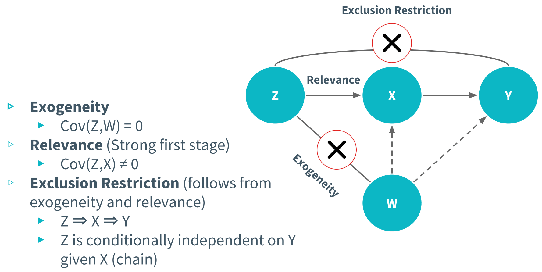
(1) First, the exogeneity assumption. Basically, what this assumption is saying is that there is no relationship between Z and all other variables which are correlated with Y and X.
(2) Second, the relevance assumption, also called the strong first stage assumption. What this means is that there is strong causal relationship between Z and X.
(3) And finally, the exclusion restriction, which states that Z affects the outcome variable, Y, only through its effect on X, meaning that the instrument does not have a direct influence on Y. It can be shown that the exclusion restriction follows from (1) and (2).
If all of these requirements are met, Z is a proper instrument. This is the first requirement to even attempt an instrumental variables analysis; otherwise we would get biased results which is what we’ve been trying to avoid all along.
The intuition of instrumental variables analysis is this. If Z is a proper instrument, variation in Z causes variation in X, without affecting the variation in W (representing all possible confounders). How do we know this? Well, we don’t for sure. We just assume it through the exogeneity and relevance assumption. The relevance assumption can be tested empirically because we have data on both Z and X. But for the exogeneity assumption, since we do not get to observe all of the confounders (precisely why controlled regression suffered from bias), we have to use some intuition, theory and domain knowledge to argue that Z is a variable that is as if random such that there is almost no chance that the instrument is correlated with other factors besides X. If exogeneity holds, then what we can do is calculate the portion of the variation in X that is exclusively caused by variation in Z, and uncorrelated with W. In the module, we used the notation X prime, to denote the portion of X that is unaffiliated with W.
In effect, we are able to break X into two parts: a part that is correlated with W, and a part that is not. By isolating the part that is not correlated with W, we get X prime, which we can use to calculate the pure causal effect of X on Y, and not the effect of X on Y that is confounded by W. To actually calculate the causal effect of X on Y, we run what is called a two-stage least squares regression, and it’s called this name because there’s two stages of regressions we have to run.
(1) The first stage involves the regression of X on Z. The interpretation? We want the portion of X that is solely explained by Z. We called this X prime. Running the first stage regression can give us the predicted values of X, solely attributed to just Z; this is the same of getting just the variation in X, attributed to variation in Z.
(2) The second stage involves the regression of Y on the X prime that we derived from the first stage. The interpretation? Well, the coefficient on X prime is the magnitude of the unbiased causal effect of X on Y that we are looking for. This coefficient is also called the two stage least squares estimator. Intuitively you can think of two stage least squares regression as like crossing two bridges: the bridge from Z to X, and the bridge from X to Y.
The good news is that instrumental variables analysis allows us to estimate the causal effect of X on Y free of omitted variable bias without having actual data on the omitted variables.
And the bad news: instrumental variables are really hard to find because they have to satisfy three assumptions, two of which aren’t exactly provable.
The basic idea of regression discontinuity is that policy rules vary at some cutoff point which yields a binary outcome: receiving treatment or control.
At the college I attended, a score less than a 59 was a fail and anything at greater than or equal to 59 was a passing score.
Therefore:
Is Person A ≈ Person B, ceteris paribus?
The key insight of regression discontinuity design is this: aren’t the people right around the threshold more or less equivalent? For example, what really is the difference between a student who scores a 59.1, and a student who scores a 58.9. Sure, one gets a passing grade and the other doesn’t get a passing grade, but besides that, can we realistically imagine these two people to be different? After all, their score differences are only 0.2.
The regression discontinuity technique is based on this assumption that there’s really no systematic difference between the people who are just below and above the cutoff. Therefore, comparing the outomes of the people just under the cutoff and the outcomes of the people just above the cutoff gives us an estimate of the causal effect of the treatment. In the grading example, the treatment is receiving a passing mark.
In RDD, we’re estimating what is called a local average treatment effect (LATE). The effect pertains to users in some narrow, or “local”, range around the cutoff. This is why some people call RDD an analysis of a local randomized experiment, where people close to the cutoff are more or less randomly assigned to treatment or control.

Researcher Sandy Black answers this question by using a regression discontinuity approach to answer this question.
In the United States, children go to the school based on the location of their home. There are attendance zones which demarcate the homes which are designated for a particular school.And basically, the idea of Black’s study was to compare houses on opposite sides of a common primary schooling attendance district boundary.

The assumption she makes is that changes in school quality are discrete at boundaries, while changes in neighborhood characteristics are smooth, meaning that all unobservable neighborhood characteristics correlated with test scores are the same on each side of the border. Therefore, comparing home values of two families who live in opposite sides of the same street, but are zoned to go to different schools, would be a good estimation of people’s willingness to pay for school quality. Black describes this as the marginal willingness to pay for a better school.
Difference in differences, is a causal inference technique that works with panel data. Panel data just means that the data has a time component, and stretches over at least two periods of time. This method requires data measured from a treatment group and a control group at two or more different time periods, specifically at least one time period before “treatment”, and at least one time period after “treatment.”
The outcome in both groups, are initially measured at some point before the treatment period. Let’s just call this the pre-intervention point. The treatment group at some time T, then receives or experiences the treatment, and both groups are again measured at some point after the treatment period. Let’s call this the post-intervention point. Note that not all of the difference in outcome, between the treatment and control groups at the post-intervention point, can be explained as being an effect of the treatment, because the treatment group and control group did not start out at the same level at the pre-intervention point. The difference in differences technique therefore deducts from this total difference, the difference that would exist if neither group experienced the treatment, represented by the constant difference in outcome.
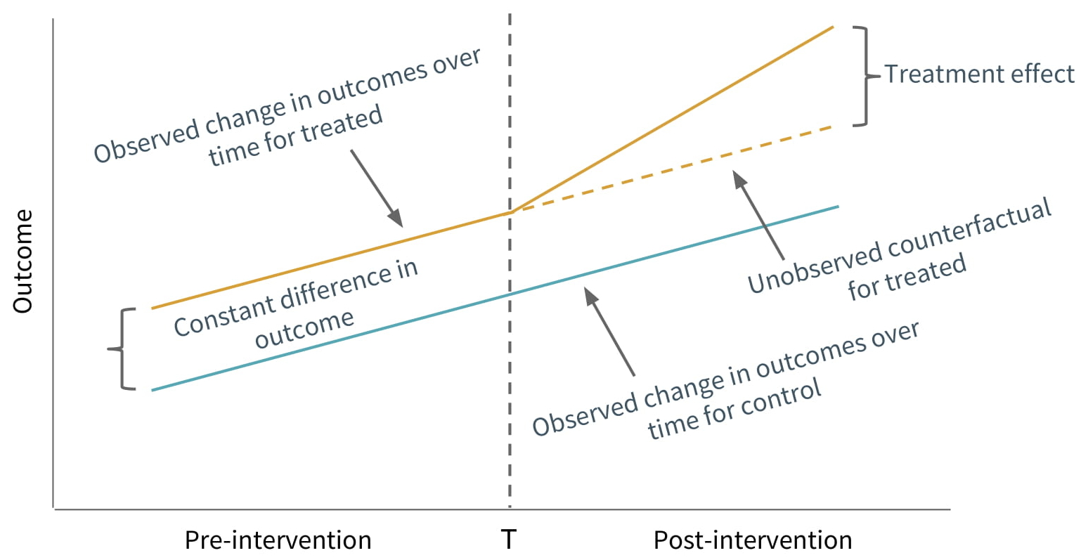
To apply difference in differences, all that is necessary is to measure outcomes in the treatment group and the control group both before and after the treatment. The difference in differences is a simple difference between two differences. Hence the name difference in differences.
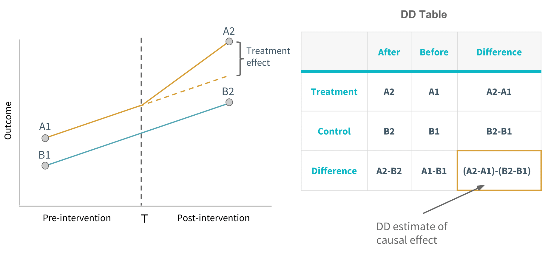
The critical assumption necessary for difference-in-differences to work is the parallel trends assumption, which says that the treatment group and the control group in the absence of treatment, follow the same trend and therefore,the difference between the treatment and control group in the absence of treatment is constant over time. What follows from the parallel trends assumption is that any deviation of the treatment group’s trend, post-intervention, from pre-intervention, is solely attributed to the treatment.
Hopefully, you have benefited from learning about causal inference. Techniques wise, we learned about randomized experiment, controlled regression, instrumental variables analysis, regression discontinuity, and difference-in-differences. These methods cover at least 90% of the empirical work that has been produced by social scientists, so I think you have pretty good coverage of the subject. Celebration time! ![]()
![]()